
For my first post I thought I’d write about some basic data classification. I’ve been going through the courses given by Carnegie Melon in the Data Science Specialization Stream to learn R and some introductory data science techniques. I recommend it.
Anyway, for the Practical Machine Learning Course they asked us to classify the how well people were performing bicep curls. The data as well as the explanation of the problem is here. We have data taken from subjects wearing sensors while they perform a bicep curl with five differing techniques (“A”, “B”, “C”, “D”, “E”). “A” corresponds to a “proper” bicep curl and the rest are differing bad techniques. The goal is to use this data to construct a classifier that can then predict the type of bicep curl using only the sensory data.
The random forest worked extremely well for this.
library(randomForest)
library(ggplot2)
library(caret)
Read in the training data
train = read.csv("pml-training.csv", stringsAsFactors = FALSE)There were a lot of columns which had many NA values and/or just missing data. I wrote a function to find the indices of these ‘useless’ columns. From inspecting the columns it seemed appropriate to remove those which did not have more than 406 entries which are not blank or NA.
#function to find index of columns with very little usable data
#from training data (blanks and NA's)
bad.cols <- function(dataframe, threshold = 406){

  #count how many non NA's are in a column
  count.non.nas =  function(x){
    sum(!is.na(x))
  }
  #find columns with too many na's
  na.cols = apply(dataframe, MARGIN = 2, count.non.nas) > threshold
  na.cols = which(na.cols == F)

  #count how many columns do not have blanks
  count.non.blanks = function(x){
    sum(!(nchar(x) == 0))
  }
  #remove columns with too many blanks
  blank.cols = apply(dataframe, MARGIN = 2, count.non.blanks) > threshold
  blank.cols = which(blank.cols == F)

  return(unique(c(na.cols, blank.cols)))
}
The indices of the unnecessary columns are
no.use.col = bad.cols(train)
no.use.col = c(1:7, no.use.col)
no.use.col
## [1] 1 2 3 4 5 6 7 18 19 21 22 24 25 27 28 29 30
## [18] 31 32 33 34 35 36 50 51 52 53 54 55 56 57 58 59 75
## [35] 76 77 78 79 80 81 82 83 93 94 96 97 99 100 103 104 105
## [52] 106 107 108 109 110 111 112 131 132 134 135 137 138 141 142 143 144
## [69] 145 146 147 148 149 150 12 13 14 15 16 17 20 23 26 69 70
## [86] 71 72 73 74 87 88 89 90 91 92 95 98 101 125 126 127 128
## [103] 129 130 133 136 139Now I prepare the data by separating out the classification column and removing the unnecessary columns. Since the classification column will not be used for analysis I remove it and keep track of it for later.
train.class = as.factor(train$classe)

train = train[, -no.use.col]
train$classe = NULL
I am using PCA to reduce dimensionality. First have to center and rescale the data. The centering and scaling comes from the training data.
#calculate mean and standard deviations for each column of train
means = colMeans(train)
sds = apply(train, 2, sd)

#center and rescale
train = as.data.frame(t((t(train) - means)/sds))

#do PCA
train.prcomp = prcomp(train, center = FALSE)

#predict using PCA
train = as.data.frame(predict(train.prcomp, newdata = train))
A plot of the first two principal components of the training set. Do they separate the data well? I don’t really see good separation…
qplot(PC1, PC2, data = train, colour = train.class)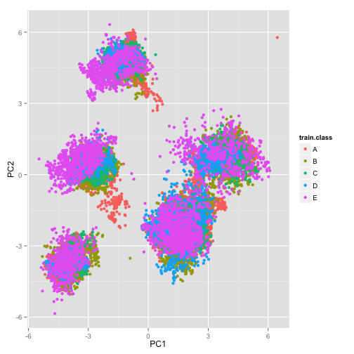
Now use the random forest to predict. I split the data into train (80%) and validation (20%) pieces. I ran random forest on the train set, used the model to predict on the validation set and calculated the error between the predicted and actual values.
train.cut = train[, c(1:25)] #use only a few of PCA's

set.seed(1224)

#split the data
index = sample(nrow(train.cut), size = 0.8*nrow(train.cut))
X = train.cut[index, ]
validation = train.cut[-index,]

#fit the model
fit = randomForest(X, train.class[index],
               importance = TRUE, ntree = 130)
predictions = predict(fit, newdata = validation)
Table of predictions on validation set against actual values and calculated cross-tabulation of observed and predicted classed.
predict.table = table(predict = predictions, true = train.class[-index])
confusionMatrix(predict.table)
## Confusion Matrix and Statistics
##
## true
## predict A B C D E
## A 1128 13 2 0 0
## B 3 750 9 0 2
## C 3 6 676 27 9
## D 0 1 7 591 4
## E 0 1 3 4 686
##
## Overall Statistics
##
## Accuracy : 0.9761
## 95% CI : (0.9708, 0.9806)
## No Information Rate : 0.2889
## P-Value [Acc > NIR] : < 2.2e-16
##
## Kappa : 0.9696
## Mcnemar's Test P-Value : NA
##
## Statistics by Class:
##
## Class: A Class: B Class: C Class: D Class: E
## Sensitivity 0.9947 0.9728 0.9699 0.9502 0.9786
## Specificity 0.9946 0.9956 0.9861 0.9964 0.9975
## Pos Pred Value 0.9869 0.9817 0.9376 0.9801 0.9885
## Neg Pred Value 0.9978 0.9934 0.9934 0.9907 0.9954
## Prevalence 0.2889 0.1964 0.1776 0.1585 0.1786
## Detection Rate 0.2874 0.1911 0.1722 0.1506 0.1748
## Detection Prevalence 0.2912 0.1946 0.1837 0.1536 0.1768
## Balanced Accuracy 0.9947 0.9842 0.9780 0.9733 0.9881